The Look-back Integrator
Basic functionality
Getting started
In epidemo/epidemo_lookback_integrator.py the class LookBackModel is
defined. Any model starts with the creation of a model object of class LookBackModel:
import epidemo
model = epidemo.LookBackModel(83000000,1.33,'2020-08-16','2021-06-01')
The number 83000000 is the total number of citizens of the country (here: Germany).
The number 1.33 is the value of \(R_0\) to be taken. The next two arguments are
the starting and ending date of the model.
Next we have to set the initial condition, i.e. the inital value of the number of new infections per day. Let’s set this to 10:
model.reset_init_infected(330)
Next we run the model:
model.run()
Note that this will start the integration only at day 5. The reason is the
nature of the lookback algorithm. The default generation time is 4 days, and the
infectivity period is 3 days (from 4-1=3 to 4+1=5 days after being
infected). That means that the lookback goes back 5 days. The
model.reset_init_infected(330) will thus set the initial condition in the
first 5 days (days 0 to 4), and we start the integration only on day 5.
If, however, you really want to have just a single day at which the number of new infections is non-zero as initial condition, you can do this with:
model.reset_init_infected(10,ndays=1)
model.run()
This will keep days 0 to 3 empty, and only set day 4 to 10 infected per day. Note, however, that this will give strong oscillations initially.
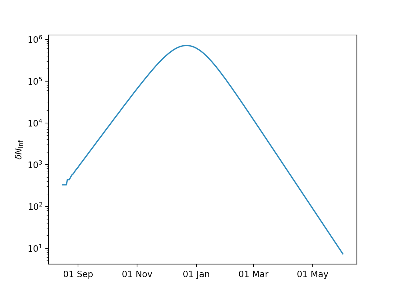
You can now plot the resulting daily new infections:
import matplotlib.pyplot as plt
days = model.time - model.time[0]
plt.figure()
plt.semilogy(days,model.Ninf_new)
plt.xlabel('Days since start')
plt.ylabel(r'$\delta N_{\mathrm{inf}}$')
plt.show()
or the cumulative number:
plt.figure()
plt.semilogy(days,model.Ninf_cum)
plt.xlabel('Days since start')
plt.ylabel(r'$N_{\mathrm{inf}}$')
plt.show()
The model.time is the time in days since 0001-01-01, called the
ordinal time. You can use Python’s datetime package to convert
any date to ordinal, for example:
import datetime
date = '2020-06-03'
d    = datetime.datetime.strptime(date,"%Y-%m-%d")
print(datetime.date(d.year, d.month, d.day).toordinal())
or back:
tord = 737579
d    = datetime.date.fromordinal(tord)
print(d.strftime("%Y-%m-%d"))
In Matplotlib you can plot the x-axis in date form:
import matplotlib.pyplot as plt
import matplotlib.dates as mdates
fig, axes = plt.subplots()
plt.semilogy(model.time,model.Ninf_new)
axes.xaxis.set_major_locator(mdates.MonthLocator([1,3,5,7,9,11]))
axes.xaxis.set_major_formatter(mdates.DateFormatter('%d %b'))
plt.ylabel(r'$\delta N_{\mathrm{inf}}$')
plt.show()
where the [1,3,5,7,9,11] is passed to the MonthLocator just to avoid
overcrowding of the x-axis by omitting each second month tick label.
Adjusting basic parameters
EpiDemo is geared toward modeling Covid-19. One of the basic parameter is the generation time, which is the mean time between successive infections. The Robert Koch Institute (RKI) uses an assumed generation time \(t_g\) of 4 days to compute the \(R_0\) value for Covid-19. The standard value of EpiDemo is therefore also set to 4. If you wish to change that to, say, 5 days, you can do that by setting it like this:
model = epidemo.LookBackModel(83000000,1.33,'2020-08-16','2021-06-01',tgen=5)
Likewise you can also adjust the time span during which a person is infectuous,
with the keyword tinf=5 (to set it to 5 days instead of the default of 3 days).
This value (tinf=5) sets \(g_0=t_g-2\) and \(g_1=t_g+2\).
Computing secondary quantities
Once you ran the model, you can post-process the results, for instance by computing various secondary quantities.
Reported number of cases
You can compute the expected number of reported new cases per day in the following way:
model.regist_meandelay = 10
model.regist_spread    = 13
model.regist_fraction  = 0.5
model.compute_positive_registrations()
where model.regist_meandelay is the mean delay between becoming infected and
the case being reported (in days), model.regist_spread is the spread of this
(in days), meaning that in this example an average will be taken between 10-6=4
days and 10+6=16 days after infection. model.regist_fraction is the fraction
of cases actually reported. It goes without saying that everything depends on the
settings of these three parameters. The stated values are rough estimates, and
should not be relied on.
Note that if these parameters are not set explicitly, then default values are taken. They may get updated in successive versions of this code.
The result is stored in model.Ninfreg_new for the new cases per day and
model.Ninfreg_cum for the cumulative of that. So here you can compare the
reported cases with the true ones:
import matplotlib.pyplot as plt
import matplotlib.dates as mdates
import epidemo
model = epidemo.LookBackModel(83000000,1.33,'2020-08-16','2021-06-01')
model.reset_init_infected(330)
model.run()
model.regist_meandelay = 10
model.regist_spread    = 13
model.regist_fraction  = 0.5
model.compute_positive_registrations()
fig, axes = plt.subplots()
plt.semilogy(model.time,model.Ninf_new,label='Real cases')
plt.semilogy(model.time,model.Ninfreg_new,':',label='Reported cases')
axes.xaxis.set_major_locator(mdates.MonthLocator([1,3,5,7,9,11]))
axes.xaxis.set_major_formatter(mdates.DateFormatter('%d %b'))
plt.ylabel(r'$\delta N_{\mathrm{inf}}$')
plt.legend()
plt.show()
It is the dotted curve that should be compared to the reported cases in the national databases.
Required ICU beds
Likewise you can compute the expected number of intensive care unit (ICU) beds:
model.icu_meandelay    = 12
model.icu_spread       = 7
model.icu_meanduration = 10
model.icu_fraction     = 0.015
model.compute_icu_occupation()
where model.icu_meandelay is the mean delay between becoming infected and
being delivered into intensive care (in days), model.icu_spread is the
spread of this (in days), meaning that in this example an average will be taken
between 12-3=9 days and 12+3=15 days after infection. model.icu_fraction is
the fraction of infected people arriving at an ICU. model.icu_meanduration
is the mean duration of a stay on ICU. It goes without saying that everything
depends on the settings of these four parameters. The stated values are rough
estimates, and should not be relied on.
Note that if these parameters are not set explicitly, then default values are taken. They may get updated in successive versions of this code.
The result is stored in model.Nicu, which is the number of ICU beds
expected to be occupied by patients of the epidemic. Example plot:
import matplotlib.pyplot as plt
import matplotlib.dates as mdates
import epidemo
model = epidemo.LookBackModel(83000000,1.33,'2020-08-16','2021-06-01')
model.reset_init_infected(330)
model.run()
model.icu_meandelay    = 12
model.icu_spread       = 7
model.icu_meanduration = 10
model.icu_fraction     = 0.015
model.compute_icu_occupation()
fig, axes = plt.subplots()
plt.semilogy(model.time,model.Ninf_new,label='Real cases')
plt.semilogy(model.time,model.Nicu,label='ICU beds occupied')
axes.xaxis.set_major_locator(mdates.MonthLocator([1,3,5,7,9,11]))
axes.xaxis.set_major_formatter(mdates.DateFormatter('%d %b'))
plt.ylabel(r'$\delta N_{\mathrm{inf}}$')
plt.legend()
plt.show()
Fatalities
Likewise you can compute the expected number of fatalities:
model.fatal_meandelay    = 15
model.fatal_spread       = 9
model.fatal_fraction     = 0.005
model.compute_fatalities()
where model.fatal_meandelay is the mean delay between becoming infected and
dying (in days), model.fatal_spread is the
spread of this (in days), meaning that in this example an average will be taken
between 15-4=11 days and 15+4=19 days after infection. model.fatal_fraction is
the fraction of infected people dying. It goes without saying that everything
depends on the settings of these four parameters. The stated values are rough
estimates, and should not be relied on.
Note that if these parameters are not set explicitly, then default values are taken. They may get updated in successive versions of this code.
The result is stored in model.Nfatal_new, for the new fatalities per day,
and model.Nfatal_cum for the cumulative number. Example plot:
import matplotlib.pyplot as plt
import matplotlib.dates as mdates
import epidemo
model = epidemo.LookBackModel(83000000,1.33,'2020-08-16','2021-06-01')
model.reset_init_infected(330)
model.run()
model.fatal_meandelay    = 15
model.fatal_spread       = 9
model.fatal_fraction     = 0.005
model.compute_fatalities()
fig, axes = plt.subplots()
plt.semilogy(model.time,model.Ninf_new,label='New cases',color='C0')
plt.semilogy(model.time,model.Nfatal_new,label='New fatalities',color='C3')
axes.xaxis.set_major_locator(mdates.MonthLocator([1,3,5,7,9,11]))
axes.xaxis.set_major_formatter(mdates.DateFormatter('%d %b'))
plt.ylabel(r'$\delta N_{\mathrm{inf}}$')
plt.legend()
plt.show()
Multi-group model
Setting up a multi-group model is only marginally more complex than setting up a single-group model. Here is an example:
import epidemo
Npoptot = 83000000
frac    = 0.1
Npop    = [Npoptot*frac,Npoptot*(1-frac)]
model = epidemo.LookBackModel(Npop,[[1.23,0.01],[0.1,0.90]],'2020-08-16','2021-06-01')
model.reset_init_infected([10,1300])
model.run()
Plotting the results:
import matplotlib.pyplot as plt
import matplotlib.dates as mdates
fig, axes = plt.subplots()
plt.semilogy(model.time,model.Ninf_new[:,0],label='Group 0')
plt.semilogy(model.time,model.Ninf_new[:,1],label='Group 1')
axes.xaxis.set_major_locator(mdates.MonthLocator([1,3,5,7,9,11]))
axes.xaxis.set_major_formatter(mdates.DateFormatter('%d %b'))
plt.ylabel(r'$\delta N_{\mathrm{inf}}$')
plt.legend()
plt.show()
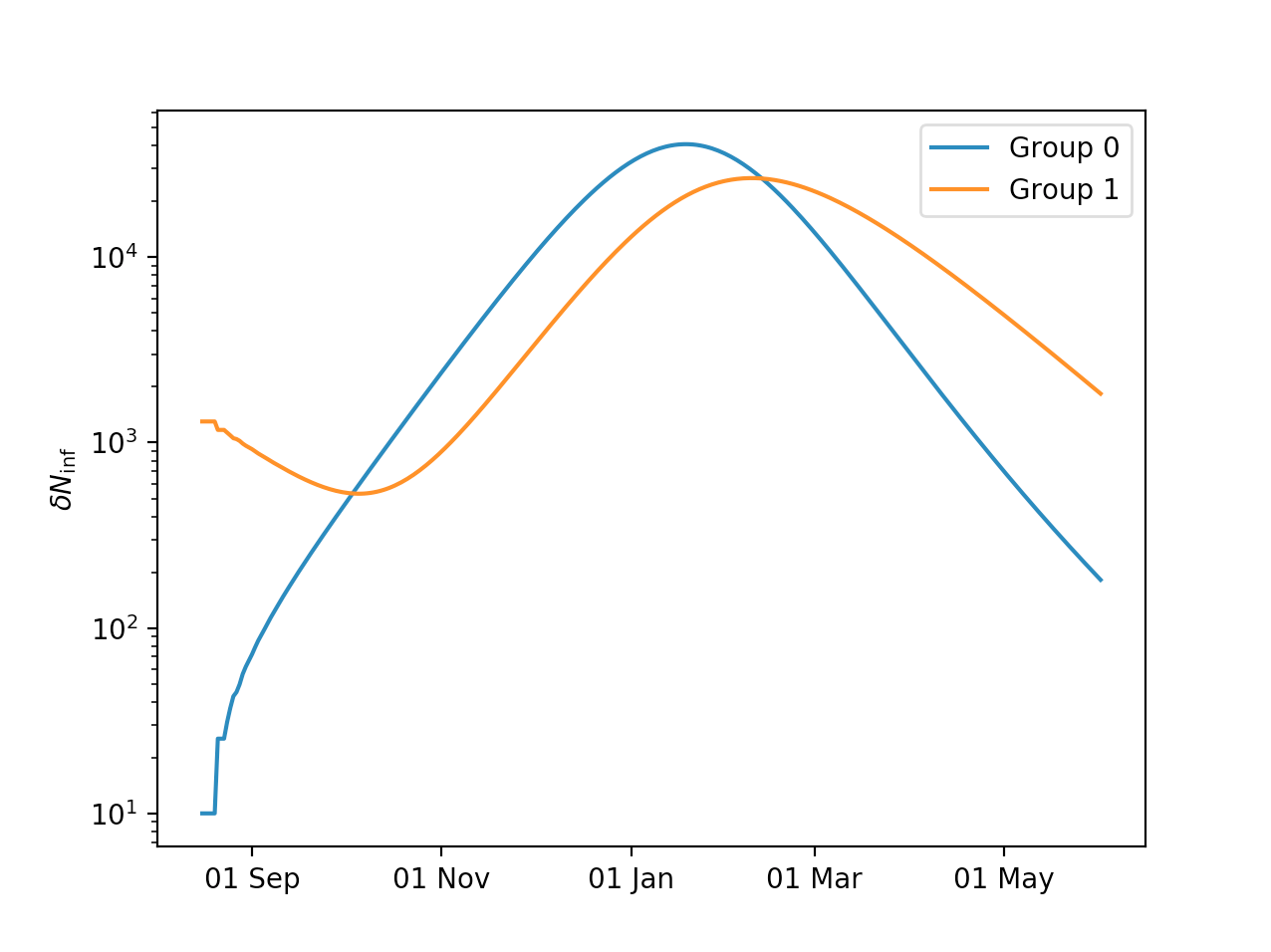
One can see how group 1 is being “pulled along” by the outbreak in group 0.